teaching_llm_applications
Week 18 — Introduction to Reinforcement Learning (Short Primer)
Overview
This is a quick primer on reinforcement learning (RL) — just enough to understand why RLHF, PPO, DPO, and GRPO are shaped the way they are. It is not meant to be comprehensive; see the further reading if you want the full theory.
1. What Is RL?
In supervised learning, you have labelled (input, correct output) pairs. In RL, an agent takes actions in an environment, receives a reward, and learns to act so as to maximise cumulative reward over time — without ever being told the “correct” action directly.
Agent observes state → picks an action → environment gives a reward
                 and a new state → repeat
The hard part: rewards can be delayed and sparse, so the agent must figure out which past actions deserve credit for a later reward (the credit assignment problem).
1.1 The Agent-Environment Loop
In supervised learning, you have labelled (input, correct output) pairs. In RL, an agent takes actions in an environment, receives a reward, and learns to act so as to maximise cumulative reward over time — without ever being told the “correct” action directly.
        ┌─────────────┐
   a_t  │             │  s_t, r_t
  ──────▶   Agent      │◀──────────
        │             │
        └─────────────┘
              │  a_t
              ▼
        ┌─────────────┐
        │ Environment │
        └─────────────┘
              │  s_{t+1}, r_{t+1}
              ▼
            (repeat)
Agent observes state → picks an action → environment gives a reward
                 and a new state → repeat
At each timestep t:
- The agent observes state s_t.
- The agent selects action a_t according to its policy π.
- The environment transitions to state s_{t+1} and emits reward r_{t+1}.
- The cycle repeats.
1.2 Why RL Matters for LLMs
-
RLHF (Week 13):
-
Concept 🧩 🚀 the LLM is the policy;
-
Concept 🧩 🚀 Policy network is the transformer;
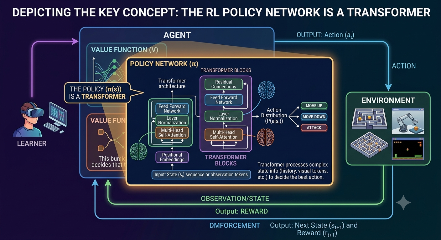
- the “environment” is a single-step bandit problem (generate a response, receive a reward, episode ends).
- GRPO / RLOO (Week 13): group-relative variants of policy gradient methods for reasoning tasks.
- Agents (Week 10): the LLM acts in a genuinely multi-step environment with tools, observations, and delayed rewards.
- DPO (Week 16): derived from the optimal solution to an RL problem with a KL constraint, even though DPO training itself involves no explicit RL loop.
Understanding classical RL is what allows you to read papers, understand why PPO is shaped the way it is, and recognise when a problem genuinely needs RL versus when supervised or preference-based methods suffice. The hard part: rewards can be delayed and sparse, so the agent must figure out which past actions deserve credit for a later reward (the credit assignment problem).
2. The Key Ingredients
- State (s): what the agent currently observes.
- Action (a): what the agent can do.
-
**Policy π(a s)*: the agent’s strategy — a (possibly probabilistic) mapping from states to actions. For an LLM, the policy *is the model: π_θ(y x). - Reward (r): a scalar signal saying how good that action was.
- Return (G): the total (discounted) reward collected over time,
G = r_1 + γr_2 + γ²r_3 + ... - Value function V(s): the expected return from state s onward, if you keep following the policy.
The goal of RL is simple to state: find the policy that maximises expected return.
3. Two Big Families of Methods
Value-based
Learn how good each state/action is (Q-learning, DQN), then act greedily with respect to that.
Policy-based
Skip the value function and directly adjust the policy’s parameters to make good actions more likely.
The simplest policy-based method is REINFORCE:
θ ← θ + α · ∇_θ log π_θ(a|s) · G
In words: if an action led to a high return, nudge the policy to make that action more likely next time. If it led to a low return, make it less likely.
This single idea — increase the probability of actions that worked out, decrease the probability of ones that didn’t, weighted by how good or bad the outcome was — is the core intuition behind every policy gradient method, including PPO.
4. Reducing Variance: Baselines and Actor-Critic
REINFORCE on its own is very noisy: the return G depends on a whole random trajectory. A simple fix is to subtract a baseline b(s) — usually an estimate of how good the state was on average:
θ ← θ + α · ∇_θ log π_θ(a|s) · (G − b(s))
This doesn’t change what the update is aiming for (still unbiased), but makes the learning signal much less noisy.
Actor-critic methods learn this baseline with a second small network (the “critic”) alongside the policy (the “actor”). This is exactly the actor/critic structure used in PPO.
5. From REINFORCE to PPO (One Sentence Each)
| Step | What it adds |
|---|---|
| REINFORCE | Basic policy gradient |
| + baseline | Less noisy updates |
| Actor-critic | Learned baseline (critic network) |
| TRPO | Limits how far one update can move the policy |
| PPO | Same idea as TRPO, implemented with simple clipping instead |
| GRPO | Like PPO, but compares a group of sampled responses instead of using a separate critic |
So when you see PPO or GRPO in the RLHF chapter (Week 13), you can now recognise it as: REINFORCE, with a learned baseline for stability, plus a safeguard against overly large updates.
6. Why This Matters for LLMs
For a single-turn chatbot response: the prompt is the state, the generated response is the action, and the reward comes from a reward model or human preference — there’s no multi-step environment, just one action per episode. This is why RLHF can often be treated as a simpler bandit problem rather than requiring full multi-step RL machinery.
For agents that take many steps (browsing, using tools, multi-turn tasks), the full RL picture — states evolving over time, delayed rewards, credit assignment — becomes much more relevant.
7. Practical This Week
See practicals/week18_practical.py:
- A tiny REINFORCE implementation on a toy bandit task.
- The same task solved with a baseline, showing the variance reduction directly in a plot.
8. Further Reading (Optional, for Depth)
- Sutton and Barto — Reinforcement Learning: An Introduction — http://incompleteideas.net/book/the-book-2nd.html
- Schulman et al. (2017) — “Proximal Policy Optimisation” — https://arxiv.org/abs/1707.06347
- OpenAI Spinning Up in Deep RL — excellent practical introduction
Discussion Questions
- In your own words, what does it mean to “increase the probability of actions that worked out”? Why is this a reasonable learning rule?
- Why does subtracting a baseline reduce variance without changing what the policy is being pushed toward?
- Why can single-turn RLHF often be treated as a bandit problem rather than a full RL problem?