Chapter 3 Computational workflow
The computational steps are outlined below. The first step is connecting to the server and loading the survival data.
library(knitr)
library(rmarkdown)
library(tinytex)
library(survival)
library(metafor)
library(ggplot2)
library(dsSurvivalClient)
require('DSI')
require('DSOpal')
require('dsBaseClient')

builder <- DSI::newDSLoginBuilder()

builder$append(server="server1", url="https://opal-sandbox.mrc-epid.cam.ac.uk",
                user="dsuser", password="P@ssw0rd",
               table = "SURVIVAL.EXPAND_NO_MISSING1")

builder$append(server="server2", url="https://opal-sandbox.mrc-epid.cam.ac.uk",
               user="dsuser", password="P@ssw0rd",
               table = "SURVIVAL.EXPAND_NO_MISSING2")

builder$append(server="server3", url="https://opal-sandbox.mrc-epid.cam.ac.uk",
               user="dsuser", password="P@ssw0rd",
               table = "SURVIVAL.EXPAND_NO_MISSING3")

logindata <- builder$build()

connections <- DSI::datashield.login(logins = logindata, assign = TRUE, symbol = "D")
3.1 Creating server-side variables for survival analysis
We now outline the steps for analysing survival data.
We show this using synthetic data. There are 3 data sets that are held on the same server but can be considered to be on separate servers/sites.
The cens variable has the event information and the survtime variable has the time information. There is also age and gender information in the variables named age and female, respectively.
We will look at how age and gender affect survival time and then meta-analyze the hazard ratios from the survival model.
- make sure that the outcome variable is numeric
ds.asNumeric(x.name = "D$cens",
             newobj = "EVENT",
             datasources = connections)

ds.asNumeric(x.name = "D$survtime",
             newobj = "SURVTIME",
datasources = connections)- convert time id variable to a factor
- create in the server-side the log(survtime) variable
- create start time variable
3.2 Create survival object and call ds.coxph.SLMA()
There are two options to generate the survival object. You can generate it separately or in line.
If a survival object is generated separately, it is stored on the server and can be used later in an assign function ( ds.coxphSLMAassign() ). The motivation for creating the model on the server side is inspired from the ds.glmassign functions. This allows the survival model to be stored on the server and can be used later for diagnostics.
- use constructed Surv object in ds.coxph.SLMA()
dsSurvivalClient::ds.Surv(time='STARTTIME', time2='ENDTIME',
                      event = 'EVENT', objectname='surv_object',
                      type='counting')

coxph_model_full <- dsSurvivalClient::ds.coxph.SLMA(formula = 'surv_object~D$age+D$female')- use direct inline call to survival::Surv()
dsSurvivalClient::ds.coxph.SLMA(formula = 'survival::Surv(time=SURVTIME,event=EVENT)~D$age+D$female',
                                dataName = 'D',
datasources = connections)- call with survival::strata()
The strata() option allows us to relax some of the proportional hazards assumptions. It allows fitting of a separate baseline hazard function within each strata.
3.3 Diagnostics for Cox proportional hazards models
We have also created functions to test for the assumptions of Cox proportional hazards models. This requires a call to the function ds.cox.zphSLMA. Before the call, a server-side object has to be created using the assign function ds.coxphSLMAassign().
All the function calls are shown below:
dsSurvivalClient::ds.coxphSLMAassign(formula = 'surv_object~D$age+D$female',
                            objectname = 'coxph_serverside')

dsSurvivalClient::ds.cox.zphSLMA(fit = 'coxph_serverside')

dsSurvivalClient::ds.coxphSummary(x = 'coxph_serverside')
These diagnostics can allow an analyst to determine if the proportional hazards assumption in Cox proportional hazards models is satisfied. If the p-values shown below are greater than 0.05 for any co-variate, then the proportional hazards assumption is correct for that co-variate.
If the proportional hazards assumptions are violated (p-values less than 0.05), then the analyst will have to modify the model. Modifications may include introducing strata or using time-dependent covariates. Please see the links below for more information on this:
https://stats.stackexchange.com/questions/317336/interpreting-r-coxph-cox-zph
https://stats.stackexchange.com/questions/144923/extended-cox-model-and-cox-zph/238964#238964
A diagnostic summary is shown below.
## surv_object~D$age+D$female## NULL## $server1
## chisq df p
## D$age 1.022 1 0.31
## D$female 0.364 1 0.55
## GLOBAL 1.239 2 0.54
##
## $server2
## chisq df p
## D$age 2.26 1 0.13
## D$female 1.96 1 0.16
## GLOBAL 3.68 2 0.16
##
## $server3
## chisq df p
## D$age 15.27 1 9.3e-05
## D$female 8.04 1 0.0046
## GLOBAL 23.31 2 8.7e-06## $server1
## Call:
## survival::coxph(formula = formula, data = dataTable, weights = weights,
## ties = ties, singular.ok = singular.ok, model = model, x = x,
## y = y)
##
## n= 2060, number of events= 426
##
## coef exp(coef) se(coef) z Pr(>|z|)
## D$age 0.041609 1.042487 0.003498 11.894 < 2e-16 ***
## D$female1 -0.660002 0.516850 0.099481 -6.634 3.26e-11 ***
## ---
## Signif. codes: 0 '***' 0.001 '**' 0.01 '*' 0.05 '.' 0.1 ' ' 1
##
## exp(coef) exp(-coef) lower .95 upper .95
## D$age 1.0425 0.9592 1.0354 1.0497
## D$female1 0.5169 1.9348 0.4253 0.6281
##
## Concordance= 0.676 (se = 0.014 )
## Likelihood ratio test= 170.7 on 2 df, p=<2e-16
## Wald test = 168.2 on 2 df, p=<2e-16
## Score (logrank) test = 166.3 on 2 df, p=<2e-16
##
##
## $server2
## Call:
## survival::coxph(formula = formula, data = dataTable, weights = weights,
## ties = ties, singular.ok = singular.ok, model = model, x = x,
## y = y)
##
## n= 1640, number of events= 300
##
## coef exp(coef) se(coef) z Pr(>|z|)
## D$age 0.04067 1.04151 0.00416 9.776 < 2e-16 ***
## D$female1 -0.62756 0.53389 0.11767 -5.333 9.66e-08 ***
## ---
## Signif. codes: 0 '***' 0.001 '**' 0.01 '*' 0.05 '.' 0.1 ' ' 1
##
## exp(coef) exp(-coef) lower .95 upper .95
## D$age 1.0415 0.9601 1.0331 1.0500
## D$female1 0.5339 1.8730 0.4239 0.6724
##
## Concordance= 0.674 (se = 0.017 )
## Likelihood ratio test= 117.8 on 2 df, p=<2e-16
## Wald test = 115.2 on 2 df, p=<2e-16
## Score (logrank) test = 116.4 on 2 df, p=<2e-16
##
##
## $server3
## Call:
## survival::coxph(formula = formula, data = dataTable, weights = weights,
## ties = ties, singular.ok = singular.ok, model = model, x = x,
## y = y)
##
## n= 2688, number of events= 578
##
## coef exp(coef) se(coef) z Pr(>|z|)
## D$age 0.042145 1.043045 0.003086 13.655 < 2e-16 ***
## D$female1 -0.599238 0.549230 0.084305 -7.108 1.18e-12 ***
## ---
## Signif. codes: 0 '***' 0.001 '**' 0.01 '*' 0.05 '.' 0.1 ' ' 1
##
## exp(coef) exp(-coef) lower .95 upper .95
## D$age 1.0430 0.9587 1.0368 1.0494
## D$female1 0.5492 1.8207 0.4656 0.6479
##
## Concordance= 0.699 (se = 0.011 )
## Likelihood ratio test= 227.9 on 2 df, p=<2e-16
## Wald test = 228.4 on 2 df, p=<2e-16
## Score (logrank) test = 229.4 on 2 df, p=<2e-163.4 Summary of survival objects
We can also summarize a server-side object of type survival::Surv() using a call to ds.coxphSummary(). This will provide a non-disclosive summary of the server-side object. The server-side survival object can be created using ds.coxphSLMAassign(). An example call is shown below:
3.5 Meta-analyze hazard ratios
We now outline how the hazard ratios from the survival models are meta-analyzed. We use the metafor package for meta-analysis. We show the summary of an example meta-analysis and a forest plot below. The forest plot shows a basic example of meta-analyzed hazard ratios from a survival model (analyzed in dsSurvivalClient).
The log-hazard ratios and their standard errors from each study can be found after running ds.coxphSLMA()
The hazard ratios can then be meta-analyzed by running the commands shown below. These commands get the hazard ratios correspondng to age in the survival model.
input_logHR = c(coxph_model_full$server1$coefficients[1,2],
        coxph_model_full$server2$coefficients[1,2],
        coxph_model_full$server3$coefficients[1,2])

input_se    = c(coxph_model_full$server1$coefficients[1,3],
        coxph_model_full$server2$coefficients[1,3],
        coxph_model_full$server3$coefficients[1,3])

meta_model <- metafor::rma(input_logHR, sei = input_se, method = 'REML')
A summary of this meta-analyzed model is shown below.
##
## Random-Effects Model (k = 3; tau^2 estimator: REML)
##
##   logLik  deviance       AIC       BIC      AICc
##   9.3824  -18.7648  -14.7648  -17.3785   -2.7648
##
## tau^2 (estimated amount of total heterogeneity): 0 (SE = 0.0000)
## tau (square root of estimated tau^2 value):      0
## I^2 (total heterogeneity / total variability):   0.00%
## H^2 (total variability / sampling variability):  1.00
##
## Test for Heterogeneity:
## Q(df = 2) = 0.0880, p-val = 0.9569
##
## Model Results:
##
## estimate      se      zval    pval   ci.lb   ci.ub
##   1.0425  0.0020  515.4456  <.0001  1.0385  1.0465  ***
##
## ---
## Signif. codes:  0 '***' 0.001 '**' 0.01 '*' 0.05 '.' 0.1 ' ' 1
We now show a forest plot with the meta-analyzed hazard ratios. The hazard ratios come from the dsSurvivalClient function ds.coxphSLMA(). The plot shows the coefficients for age in the survival model. The command is shown below.
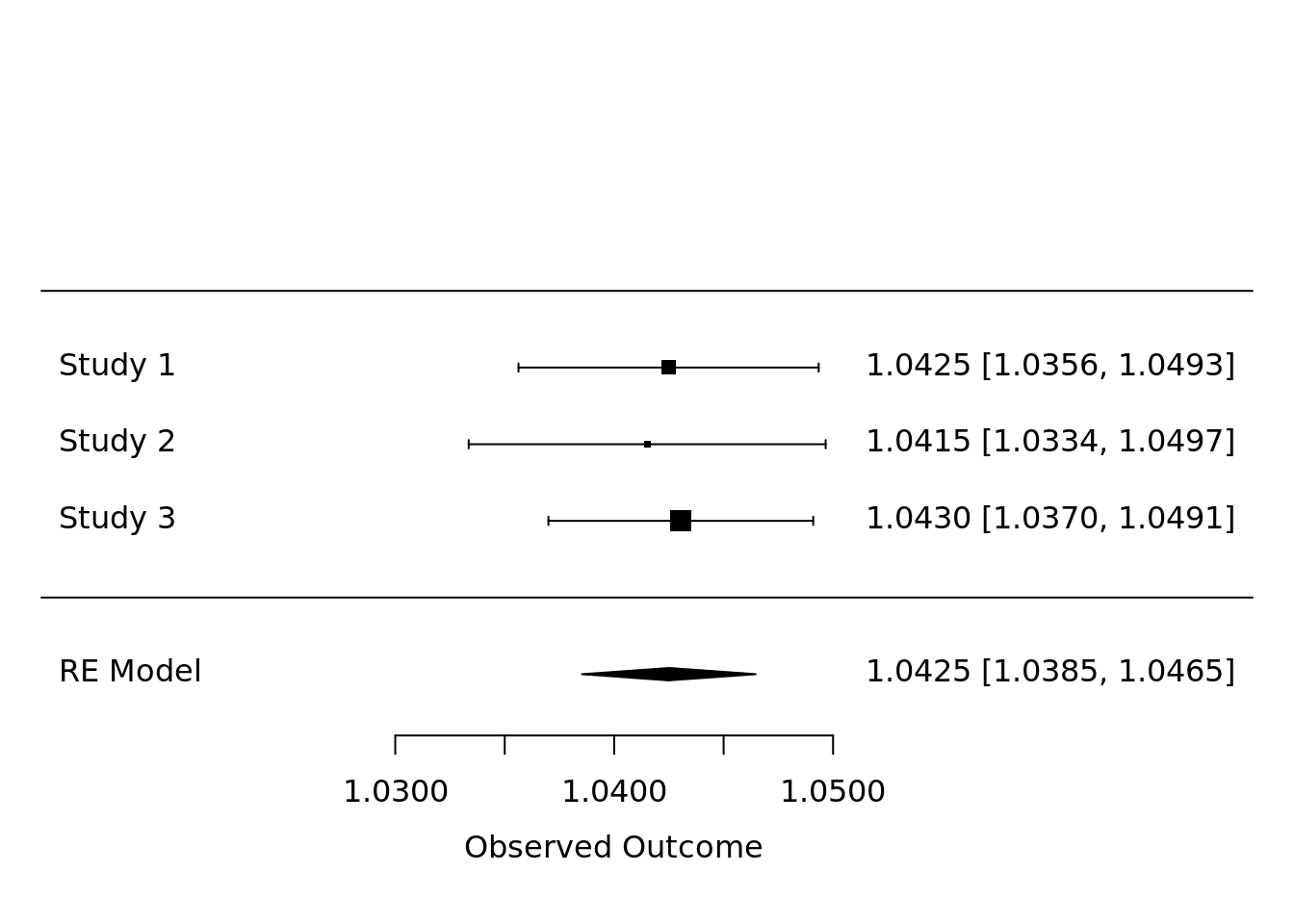
Figure 3.1: Example forest plot of meta-analyzed hazard ratios.
3.6 Plotting of privacy-preserving survival curves
We also plot privacy preserving survival curves.
 dsSurvivalClient::ds.survfit(formula='surv_object~1', objectname='survfit_object')
 dsSurvivalClient::ds.plotsurvfit(formula = 'survfit_object')
## NULL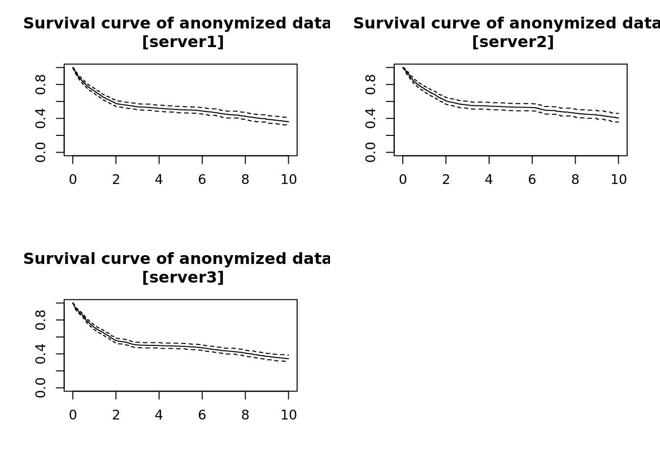
Figure 3.2: Privacy preserving survival curves.
## $server1
## Call: survfit(formula = formula)
##
## records       n  events  median 0.95LCL 0.95UCL
## 2060.00  886.00  426.00    5.24    3.13    6.84
##
## $server2
## Call: survfit(formula = formula)
##
## records       n  events  median 0.95LCL 0.95UCL
## 1640.00  659.00  300.00    6.56    4.57    8.45
##
## $server3
## Call: survfit(formula = formula)
##
## records       n  events  median 0.95LCL 0.95UCL
## 2688.00 1167.00  578.00    3.86    2.59    6.15
Finally, once you have finished your analysis, you can disconnect from the server(s) using the following command: