teaching_llm_applications

Resource accounting

• Stanford CS336 course Lecture 2

• Lecture notes

• float 32 representation

• Python code

• 🎮 Practicals and here

    import torch
    x = torch.zeros(4, 8)  
    assert x.dtype == torch.float32  # Default type
    assert x.numel() == 4 * 8
    assert x.element_size() == 4  # Float is 4 bytes
    assert get_memory_usage(x) == 4 * 8 * 4  # 128 bytes
    # One matrix in the feedforward layer of GPT-3:
    assert get_memory_usage(torch.empty(12288 * 4, 12288)) == 2304 * 1024 * 1024  # 2.3 GB 

• reduce storage quantization

• float 16 practicals

x = torch.zeros(4, 8, dtype=torch.float16)  
    assert x.element_size() == 2
    However, the dynamic range (especially for small numbers) isn't great.
    x = torch.tensor([1e-8], dtype=torch.float16)  
    assert x == 0  # Underflow!
    

• If this happens when you train, you can get instability.

• bfloat16

• fp8

• training with fp8, float16 and bfloat16 can lead to instabilities

• automatic mixed precision AMP

• cast into bf16 (safe for matmul not exp)

• Concept 🧩 🚀 Train on high precision (bf16) and then quantize

• 🤔 Is quantization at training time or inference time?

• move tensors to GPUs

• einops tutorial

• 💡 generalized matrix multiplication where dimensions are named

def einops_motivation():
    #Easy to mess up the dimensions (what is -2, -1?)...
    Traditional PyTorch code:
    x = torch.ones(2, 2, 3)      # batch seq hidden  
    y = torch.ones(2, 2, 3)      # batch seq hidden  
    z = x @ y.transpose(-2, -1)  # batch seq seq  
    #Easy to mess up the dimensions (what is -2, -1?)...


def einops_einsum():
    #Einsum is generalized matrix multiplication with good bookkeeping.
    x = torch.ones(3, 4)  # seq1 hidden 
    y = torch.ones(4, 3)  # hidden seq2 
    # Old way
    z = x @ y   # seq1 seq2  
    # New (einops) way
    z = einsum(x, y, "seq1 hidden, hidden seq2 -> seq1 seq2")    

    # Let's try a more complex example...
    x = torch.ones(2, 3, 4)  # batch seq1 hidden 
    y = torch.ones(2, 3, 4)  # batch seq2 hidden 
    # Old way
    z = x @ y.transpose(-2, -1)  # batch seq1 seq2  
    # New (einops) way
    z = einsum(x, y, "batch seq1 hidden, batch seq2 hidden -> batch seq1 seq2")  
    # Dimensions that are not named in the output are summed over.  

• rearrange

• floating point operation (FLOP)

• x + y is 1 FLOP

• $x + y + z$ is 2 FLOPs

• $x @ y$ is $mnp$ FLOPs for matrices of size $(m, n)$ and $(n, p)$

• Training GPT-3 took 3.14e23 FLOPS

• Question: How long would it take to train a 70B parameter model on 15T tokens on 1024 B100s?

    total_flops = 6 * 70e9 * 15e12  
    h100_flop_per_sec = 1979e12 / 2
    mfu = 0.5
    flops_per_day = h100_flop_per_sec * mfu * 1024 * 60 * 60 * 24  
    days = total_flops / flops_per_day  

• matrix multiplication is a very costly operation in AI/ML

• B: number of points, D: dimension, K: number of outputs

• FLOPS = 2 * B * D * K

• element wise operation on a matrix M x N = O(MN) FLOPS

• MFU: Model FLOPs Utilization - how close to the theoretical maximum are we?

• FLOPS for forward pass: 2 * num_parameters * num_tokens

• Memory bound vs. Compute bound:

  The theoretical maximum number of floating point operations per second of a processor is its theoretical maximum speed. For example, an NVIDIA H100 has a theoretical maximum speed of about 2000 teraflops (that is $2 \times 10^{15}$ flop/s), where a flop may be an addition, multiplication, division, etc.

  For matrix multiplication of two matrices of shape $M \times N$ and $N \times P$, we perform $M \times N \times P$ multiplications and $M \times N \times P - M \times P$ additions. This is approximately $2MNP$ flops.

• MFU

• arithmetic intensity = flops / bytes

• it means flops per byte

• it measures how computationally intensive the operation is

• it is a measure of how effectively we use the computational resources of the processor

• Concept 🧩 🚀 Transformers have very high arithmetic intensity (so it exploits the compute resources of the processor well)

• accelerator speed and memory bandwidth

• 

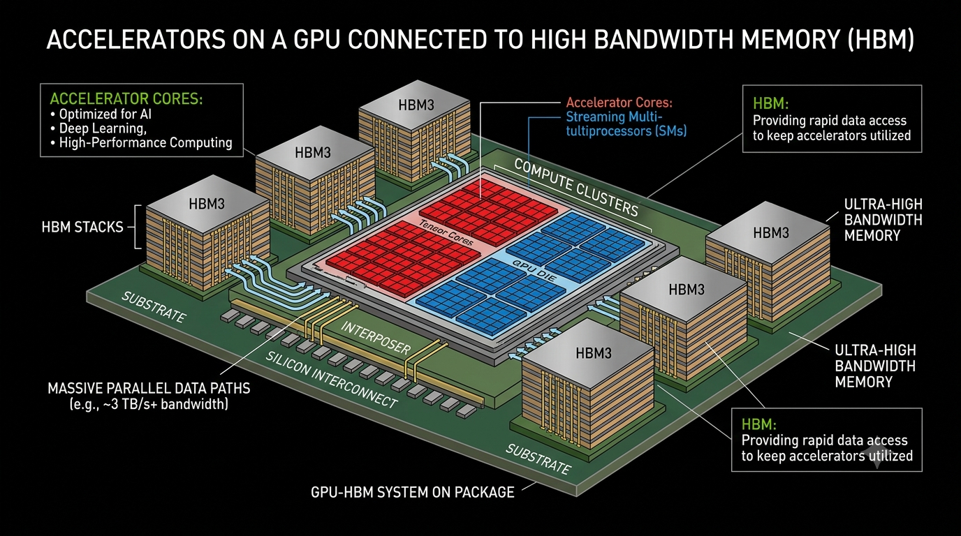
• also see chapter on GPUs

• $\text{flops/byte} = \frac{\text{peak FLOPS}}{\text{memory bandwidth in bytes/sec}}$

• If you have something in memory it needs to be moved also

• GeLU is computationally more expensive than ReLU, in GPT architecture we use GeLU

• Practical

def arithmetic_intensity_gelu():
    n = 1024
    x = torch.ones(n, dtype=torch.bfloat16, device=cuda_if_available())
    y = F.gelu(x)  # GELU(x) = 0.5 x (1 + tanh(sqrt(2/pi) (x + 0.044715 x^3)))
    bytes = (2 * n) + (2 * n)  # Read x, write y (bf16 is 2 bytes/float)
    flops = 20 * n  # tanh can approximated in various ways (e.g., polynomial)
    arithmetic_intensity = flops / bytes  
    h100_accelerator_intensity = h100_flop_per_sec / h100_bytes_per_sec  
    assert arithmetic_intensity < h100_accelerator_intensity

    # Note that GeLU does more work than ReLU per byte moved, so it has higher arithmetic intensity.
    # But still memory-bound!
    # In other words, ReLU is not faster than GeLU (when doing things in an isolated way).

• Practical

def arithmetic_intensity_dot_product():
    n = 1024
    x = torch.ones(n, dtype=torch.bfloat16, device=cuda_if_available())
    w = torch.ones(n, dtype=torch.bfloat16, device=cuda_if_available())
    y = x @ w
    bytes = (2 * n) + (2 * n) + 2  # Read x, read w, write y
    flops = 2 * n - 1  # n multiplications, n-1 additions
    arithmetic_intensity = flops / bytes  # ~1/2 
    h100_accelerator_intensity = h100_flop_per_sec / h100_bytes_per_sec  
    assert arithmetic_intensity < h100_accelerator_intensity
    # Memory-bound!

• During inference we are doing matrix vector product

• As long as we have big matrices, we are compute bound

• 💡 Inference is faster than training

• 💡 Matrix vector product is what happens in inference because we only have one input vector which we dot product with a matrix (and so inference is memory bound)

• 💡 Training transformers is compute bound and involves big matrix multiplications (and so training is compute bound)

• 🎥 Roofline plots

• Roofline plots

• Roofline plots plot the arithmetic intensity on x-axis and performance (FLOPS) on y-axis.

Deep networks cost

• Forward pass cost: 2 * data_points * num_parameters FLOPS

• Backward pass cost: 4 * data_points * num_parameters FLOPS

• Total: 6 * data_points * num_parameters FLOPS

• This is for multi-layer perceptrons but works for transformers as well (for short context length)

• for longer context length: * sequence_length factor also appears (roughly) * sequence_length^2 in the memory cost (not just compute)

• practical

def deep_linear_network():
    
    Consider a deep network with L layers and D-dimensional inputs, activations, and outputs.
    # Define the network
    D = 8  # Dimensionality of input, activations, and output
    L = 3  # Number of layers
    model = DeepNetwork(dim=D, num_layers=L).to(cuda_if_available())
    num_parameters = get_num_parameters(model)  
    assert num_parameters == (D * D) * L
    # Run the model on a batch of data
    B = 4  # Batch size
    x = torch.randn(B, D, device=cuda_if_available())  
    y = model(x)  

class Block(nn.Module):
    """Simple block that applies a linear transformation followed by a ReLU nonlinearity."""
    def __init__(self, dim: int):
        super().__init__()
        self.weight = nn.Parameter(torch.randn(dim, dim) / np.sqrt(dim))
    def forward(self, x: torch.Tensor) -> torch.Tensor:
        x = x @ self.weight  # Linear
        x = F.relu(x)        # Activation
        return x

class DeepNetwork(nn.Module):
    """Map `dim`-vector to a `dim`-vector."""
    def __init__(self, dim: int, num_layers: int):
        super().__init__()
        self.layers = nn.ModuleList([Block(dim) for i in range(num_layers)])
    def forward(self, x: torch.Tensor) -> torch.Tensor:
        # Apply all the layers sequentially
        for layer in self.layers:
            x = layer(x)  
        return x

• gradient accumulation hack: compute gradient on micro-batches and accumulate the gradients, update the parameters only once in a while (and then zero out the gradients)

• activation checkpointing

• for training we need to store all activations

• for inference we only need activations for the current layer (no gradients)

• 🤔 if you want to reduce memory, recompute activations during the backward pass (but this is slower)

Summary

• everything is in tensors (parameters, activations, gradients, optimizer state, data)

• einops

• compute vs memory bounds

• matrix multiplication is very compute intensive; element-wise operations are memory intensive

• reduce memory usage by gradient accumulation (trade-off: slower training) and activation checkpointing (trade-off: slower training)

• 🤔 How long would it take to train a 70B parameter model on 15T tokens on 1024 B100s?

This site is open source. Improve this page.