teaching_robots_navigation

1. Frames and pose

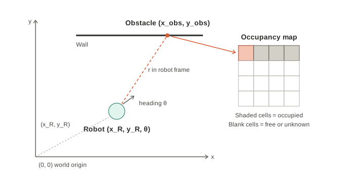
Robot pose, obstacle and occupancy map

World frame. A fixed frame with its origin at $(0, 0)$, for example a corner of the room. The map lives in this frame.

Robot pose. The robot’s position and heading in the world frame:

\[\mathbf{p} = (x_R,\; y_R,\; \theta)\]

where $\theta$ is the angle between the robot’s forward direction and the world $x$-axis.

Robot frame. A frame attached to the robot, with its origin at the robot and its $x$-axis pointing forward. A range sensor reports obstacles in this frame, written $(x_{obs}^{R},\; y_{obs}^{R})$. The superscript $R$ means “expressed in the robot frame”.

2. From robot frame to world frame

To put a measurement on the map we convert it to world coordinates. This is a rotation by $\theta$ followed by a translation by the robot’s position:

\[\begin{aligned} x_{obs} &= x_R + x_{obs}^{R}\cos\theta - y_{obs}^{R}\sin\theta \\ y_{obs} &= y_R + x_{obs}^{R}\sin\theta + y_{obs}^{R}\cos\theta \end{aligned}\]

In matrix form:

\[\begin{bmatrix} x_{obs} \\ y_{obs} \end{bmatrix} = \begin{bmatrix} x_R \\ y_R \end{bmatrix} + \begin{bmatrix} \cos\theta & -\sin\theta \\ \sin\theta & \cos\theta \end{bmatrix} \begin{bmatrix} x_{obs}^{R} \\ y_{obs}^{R} \end{bmatrix}\]

Common student errors

Forgetting the rotation (this is only valid when $\theta = 0$).
Mixing degrees and radians.
Using the wrong sign convention for $\theta$ (counter-clockwise positive is standard).

Sensor that returns range and bearing. If the sensor gives a distance $r$ and a bearing $\phi$ relative to the robot’s heading, first convert to the robot frame:

\[x_{obs}^{R} = r\cos\phi, \qquad y_{obs}^{R} = r\sin\phi\]

and then apply the transform above.

3. Occupancy maps

An occupancy grid divides the world into cells. Each cell stores whether it is occupied, free or unknown.

Update procedure for one range measurement

Convert the measurement to world coordinates $(x_{obs}, y_{obs})$ using Section 2.
Find the grid cell containing that point and mark it occupied.
Mark the cells along the ray from the robot to the obstacle as free, since the beam passed through them.
Leave cells beyond the obstacle unknown.

Probabilistic version. Real sensors are noisy, so each cell stores a probability or, more commonly, a log-odds value $\ell$ that is incremented on a hit and decremented on a miss:

\[\ell_{t}(c) = \ell_{t-1}(c) + \ell_{\text{sensor}}(c)\]

Repeated consistent readings push a cell firmly toward occupied or free, while occasional bad readings are averaged out.

4. Reactive control for a differential-drive robot

Differential-drive obstacle avoidance

Concept 🧩 🚀

obstacle_avoidance_reactive

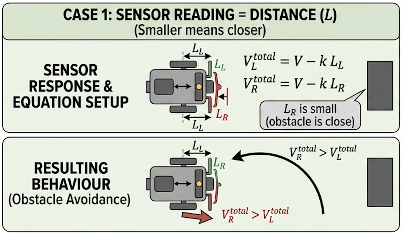
A differential-drive robot has two independently driven wheels. Let $V_L$ and $V_R$ be the left and right wheel speeds.

Equal speeds: the robot drives straight.
Right wheel faster than left: the robot turns left.
Left wheel faster than right: the robot turns right.

Constant base speed. Start from a constant forward speed for each wheel, $V_L = V_R = V$. This gives constant linear velocity when no obstacles are sensed.

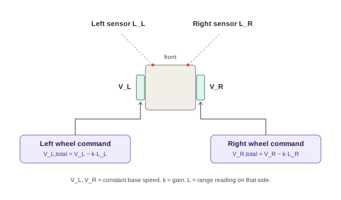
Sensor-driven correction. Each wheel’s speed is reduced by its own side’s sensor reading, scaled by a gain $k$:

\[\begin{aligned} V_L^{\text{total}} &= V_L - k\,L_L \\ V_R^{\text{total}} &= V_R - k\,L_R \end{aligned}\]

where $L_L$ and $L_R$ are the left and right sensor readings.

What does $L$ mean? This decides the behaviour

Reading $L$	Obstacle close on the right	Wheel effect	Behaviour
Distance (small when close)	$L_R$ is small	Right wheel slowed less than left	Turns left, away from the obstacle
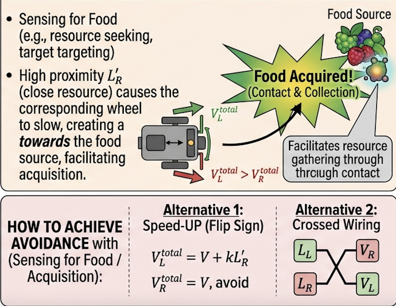
Proximity (large when close)	$L_R$ is large	Right wheel slowed more than left	Turns right, toward the obstacle

Concept 🧩 🚀

For obstacle avoidance with the equations above, use a distance reading. With a proximity reading, flip the sign (add $k\,L$ instead of subtracting)
or cross the wiring between sensors and wheels. see diagram below to use cross wiring to find food etc.

A side effect of the distance convention is that the robot drives slower in open space, because $L$ is large there. Many implementations clamp $L$ to a maximum range or subtract $k\,(L_{\max} - L)$ instead.

5. Braitenberg vehicles

The wiring above is an example of a Braitenberg vehicle, from Valentino Braitenberg’s 1984 book Vehicles: Experiments in Synthetic Psychology. These are thought experiments in which sensors are connected directly to motors, with no map, memory or planning. Different wiring produces behaviour an observer would describe in psychological terms.

Vehicle	Wiring	Behaviour
2a “fear”	Same-side sensor excites wheel	Turns away from the stimulus and speeds off
2b “aggression”	Opposite-side sensor excites wheel	Turns toward the stimulus and charges at it
3a “love”	Same-side sensor inhibits wheel	Approaches the stimulus, slows and stops facing it
3b “explorer”	Opposite-side sensor inhibits wheel	Turns away and slows near the stimulus

Teaching point. Useful, apparently purposeful behaviour needs almost no computation. This is also the clearest way to show what reactive control cannot do: it has no memory, no goals and no model of the world.

In vehicles of Type 2a, the two sensors and two wheels are connected by ipsilateral excitatory wires. If a stimulus is located in front of the vehicle and to its left, it will activate both of the vehicle’s sensors, but unequally; the left sensor is closer to the stimulus and will therefore be activated more strongly. This increased activation leads to increased activation in both wheels, but unequally; the left wheel is activated more strongly than the right. Thus the vehicle turns to the right, suggesting to Braitenberg that it “fears” the stimulus.

also connects to why nerves criss-cross the hemispheres in our brain

6. Why reactive control is not enough: motivating SLAM

Reactive controllers fail in situations such as:

Local traps: corners and dead ends where avoiding one wall points the robot at another.
No global goal: the robot cannot plan a route to a specified location.
No memory: it re-discovers the same obstacle every time.

The fix is to build and use a map. But Section 2 shows that a correct map needs a correct pose, and the robot’s pose estimate drifts because wheel odometry accumulates error. To correct the pose, the robot needs the map. This is the SLAM problem: Simultaneous Localisation And Mapping.

\[\underbrace{\text{map}}_{\text{needs pose}} \;\;\longleftrightarrow\;\; \underbrace{\text{pose}}_{\text{needs map}}\]

Typical SLAM loop

Predict the new pose from odometry (wheel encoders, IMU).
Sense the environment with range sensors or a camera.
Match the new scan against the current map to correct the pose.
Update the map using the corrected pose (Section 3).
Close loops: when the robot returns to a known place, correct accumulated drift across the whole trajectory.

Common families include filter-based SLAM (EKF, particle filters), graph-based SLAM (pose-graph optimisation) and visual SLAM.

7. Worked code example

A minimal Python sketch for the transform, occupancy update and reactive controller.

import math

def robot_to_world(x_r, y_r, theta, x_obs_R, y_obs_R):
    """Convert an obstacle point from robot frame to world frame."""
    c, s = math.cos(theta), math.sin(theta)
    x_obs = x_r + x_obs_R * c - y_obs_R * s
    y_obs = y_r + x_obs_R * s + y_obs_R * c
    return x_obs, y_obs

def mark_occupied(grid, x_obs, y_obs, cell_size):
    """Mark the grid cell containing (x_obs, y_obs) as occupied (1)."""
    col = int(x_obs // cell_size)
    row = int(y_obs // cell_size)
    if 0 <= row < len(grid) and 0 <= col < len(grid[0]):
        grid[row][col] = 1

def wheel_speeds(v_base, k, l_left, l_right):
    """Braitenberg-style control; l_* are distance readings."""
    v_left = v_base - k * l_left
    v_right = v_base - k * l_right
    return v_left, v_right

# Example: robot at (2, 2) facing 45 degrees, obstacle 3 m straight ahead
x, y = robot_to_world(2.0, 2.0, math.radians(45), 3.0, 0.0)
print(round(x, 2), round(y, 2))   # 4.12 4.12

8. Discussion questions and exercises

A robot at $(1, 1)$ with $\theta = 90^\circ$ measures an obstacle at $(2, 0)$ in its own frame. Where is the obstacle in the world frame? (Answer: $(1, 3)$.)
What happens to the map if the robot’s heading estimate is off by $5^\circ$ and the obstacle is $10\,\text{m}$ away? (Roughly $0.87\,\text{m}$ sideways error.)
Using the controller in Section 4, what happens if $L_L = L_R$? Is that enough to guarantee the robot avoids a wall head-on?
Which Braitenberg wiring would you choose for a robot that should follow a light source, and which for one that should avoid it?
Why can a Braitenberg vehicle not solve a maze, and what minimal extra ingredient would help?

9. Summary

Concept	Key idea
Pose	$(x_R, y_R, \theta)$ in the world frame
Frame transform	Rotate by $\theta$, then translate by $(x_R, y_R)$
Occupancy grid	World cut into cells, updated from each measurement
Reactive control	$V^{\text{total}} = V - k\,L$ per side; sign depends on what $L$ measures
Braitenberg vehicles	Sensor-to-motor wiring alone gives lifelike behaviour
SLAM	Pose and map must be estimated together