teaching_robots_navigation
Navigation
-
navigation and planning
-
relative to other locations
-
path planning
-
self localisation
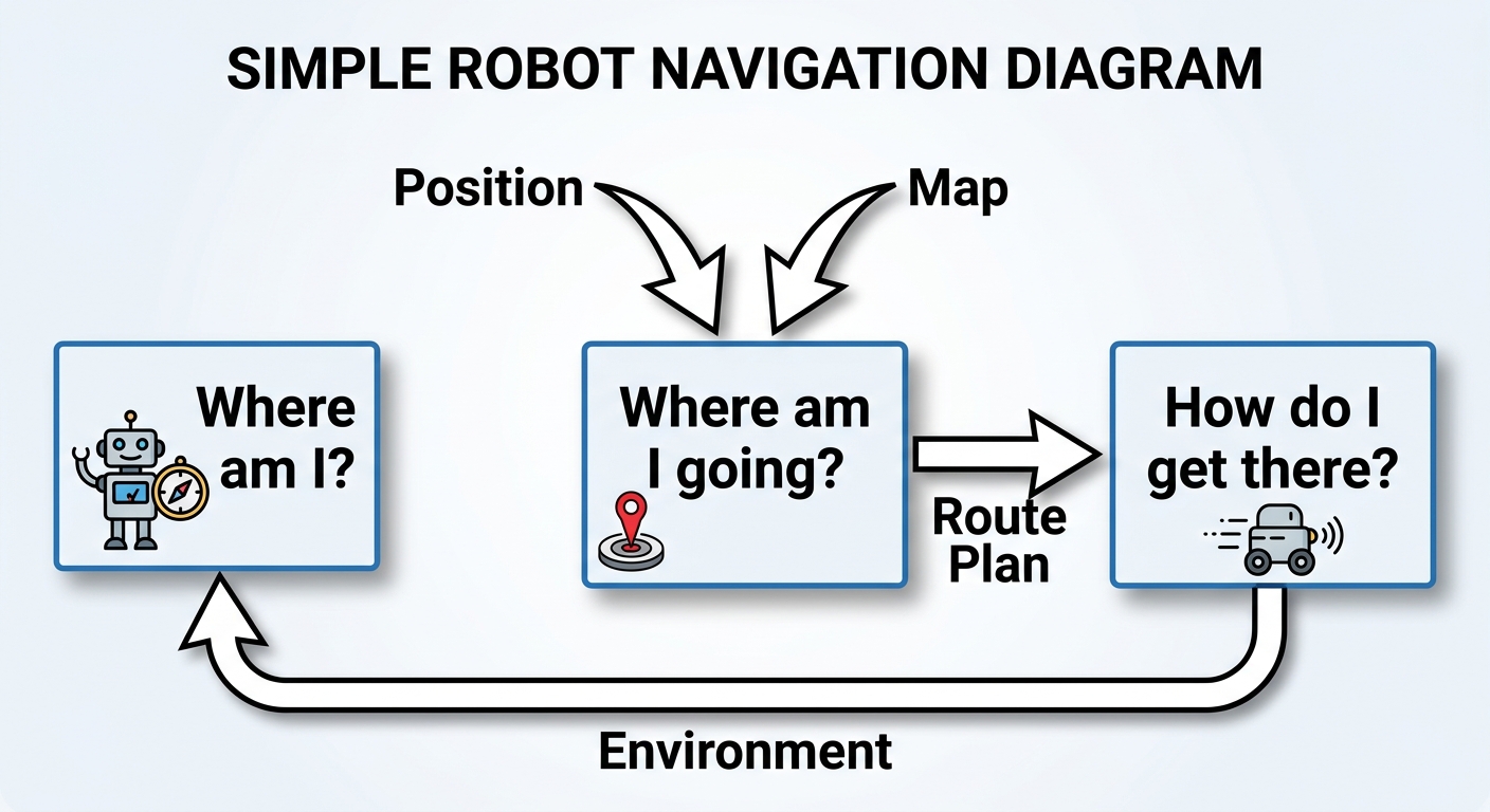
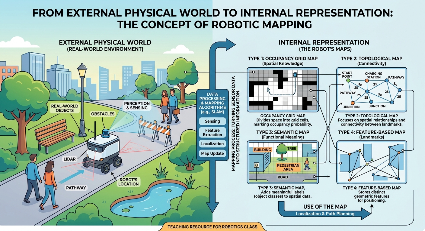
- map is a
mappingfrom the real world to some internal representation
-
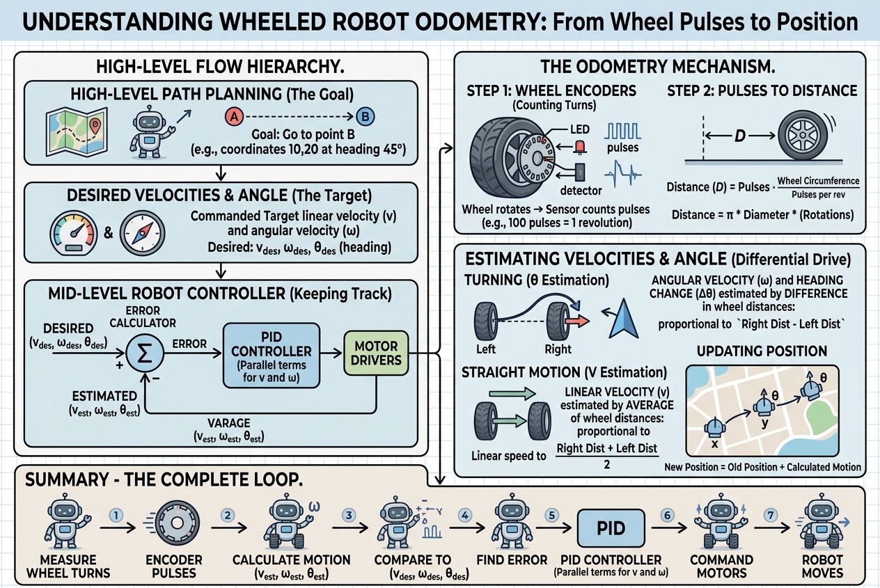
PID controller Proportional Integrative and Derivative
-
See resource on odometry
-
these get translated to right and left wheel velocities
-
this is what guides the robot from where it is to where it needs to go
-
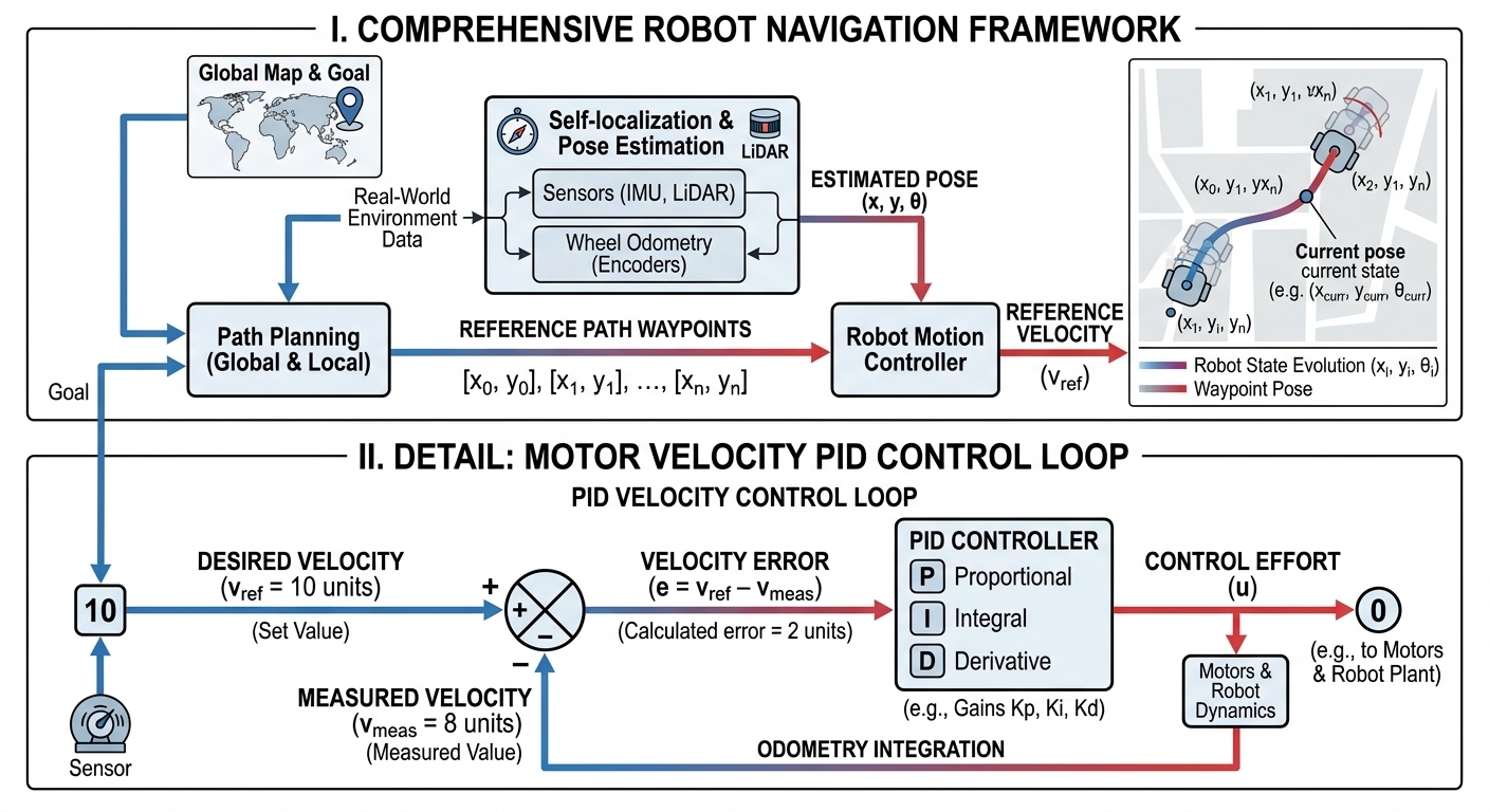
generate a series of x, y values to guide a robot
-
self localization -
path planner
-
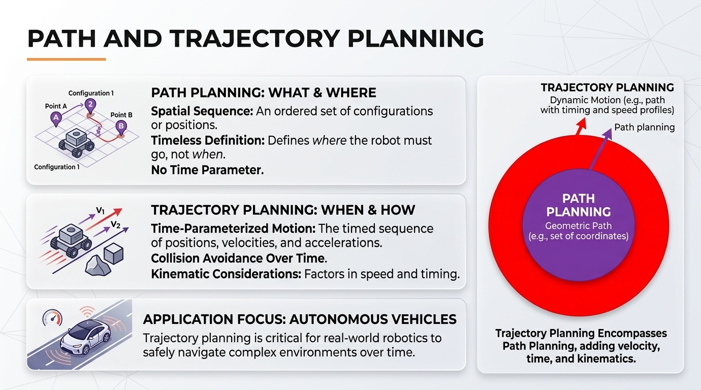
path planning is different from trajectory planning
-
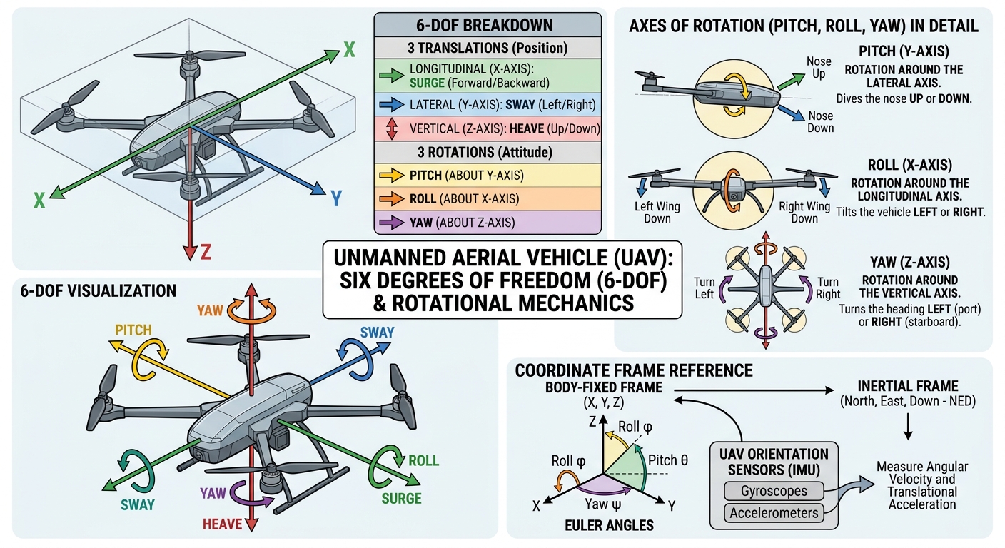
aerial drones have 6 degrees of freedom pitch, roll and yaw
-
balance shorter term goals with long term for path planning
-
path planning is a subset of trajectory planning
- some path planning techniques
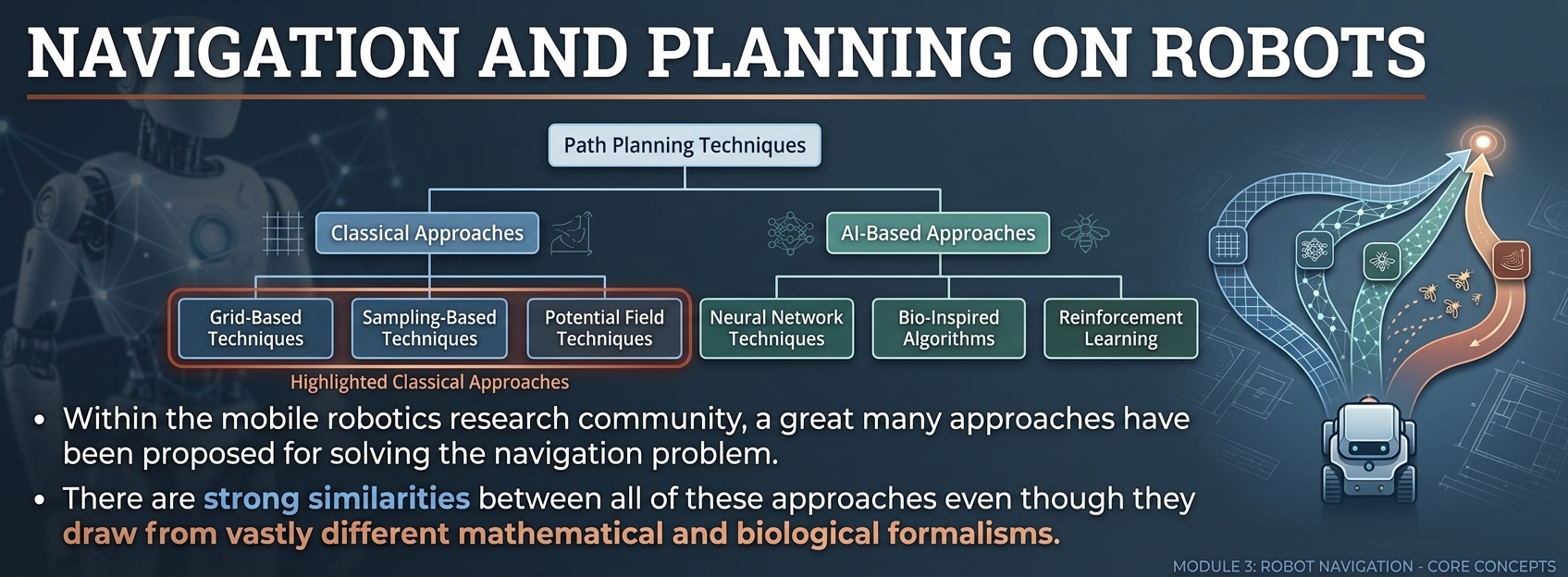
- reinforcement learning: control strategies that work get reinforced
What is required
- a global map
- robot must know where it is in the map
- start
- goal
🤔❓Challenge question (discussion in class)
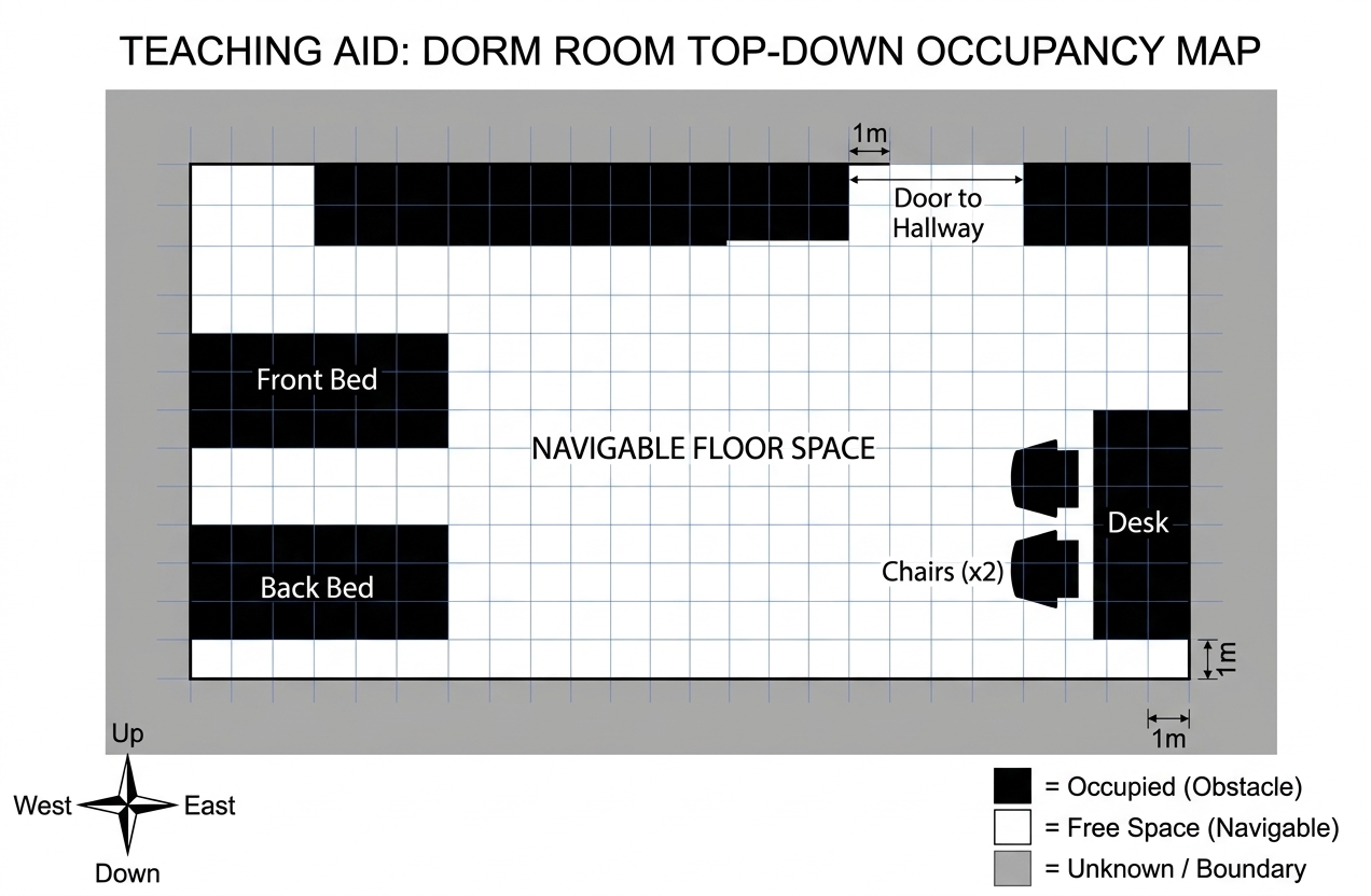
Occupancy map
-
exploration of environment
-
position estimation using robot pose
-
sensor values interpret (LIDAR, sonar, vision, etc.)
-
integration of sensor values into map (based on distance from robot and pose estimation of robot)
-
what happens to table? robot can go underneath. the choice is with you
-
divide into grids
-
binary (occupied/not occupied) within each cell
Artificial potential fields
- force that will push it away
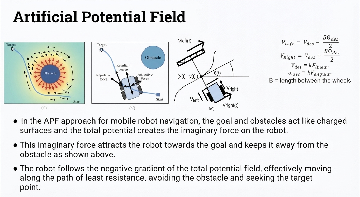
B = length between the wheels
- In the APF approach for mobile robot navigation, the goal and obstacles act like charged surfaces and the total potential creates the imaginary force on the robot.
- This imaginary force attracts the robot towards the goal and keeps it away from the obstacle as shown above.
-
The robot follows the negative gradient of the total potential field, effectively moving along the path of least resistance, avoiding the obstacle and seeking the target point.
-
🤔 ❓disadvantage
-
need to know map before you setup potential field
-
what will happen when you change target
-
all stored in memory
-
number of cells required ; how will this scale as you go to bigger environments
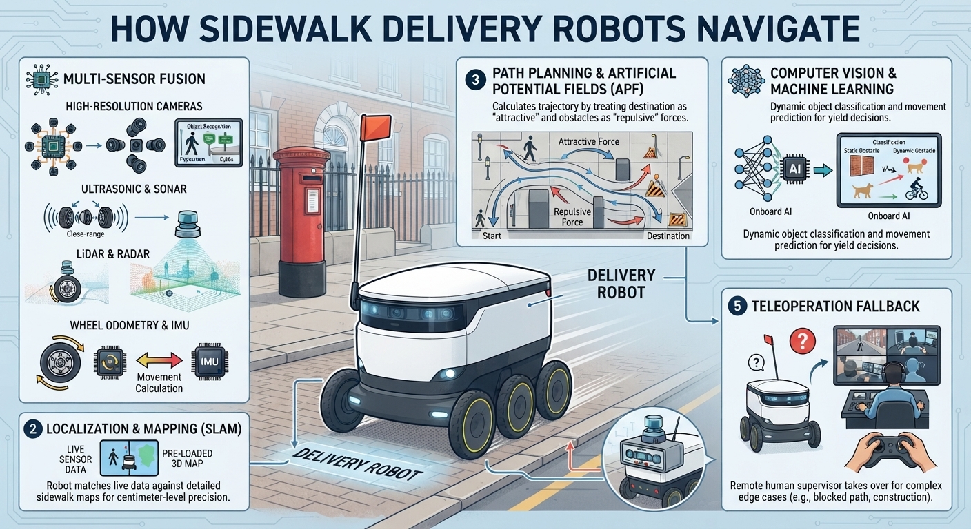
- 🤔 ❓how does this delivery robot navigate?
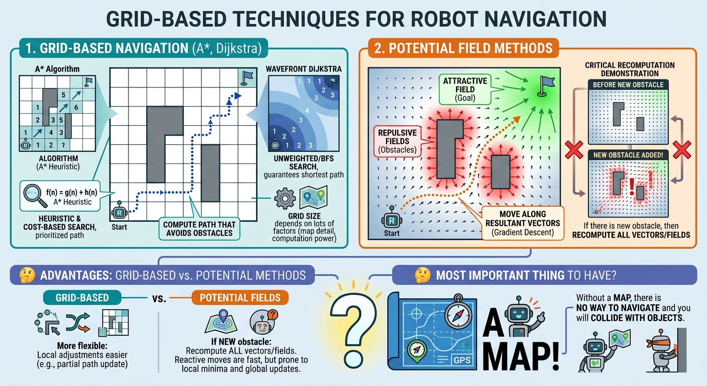
Grid based techniques for robot navigation
-
A* algorithm
-
Dijkstra
-
compute path that avoids obstacles
-
grid size depends on lots of factors
-
🤔 ❓what are the advantages of grid based vs. potential methods
-
more flexible
-
if there is new obstacle, then recompute all vectors/fields
-
🤔 ❓what is the most important thing to have in order to have a successful navigating robot?
-
Answer: you need a map
-
without a map, there is no way to navigate and collide with object
Sample based planning
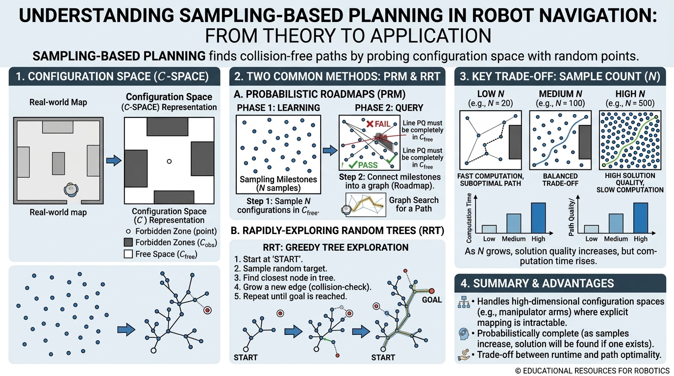
Sampling-based motion planning is a fundamental approach in modern robotics used to find collision-free paths in complex or high-dimensional environments. Rather than explicitly computing the exact boundaries of all obstacles, sampling-based algorithms approximate the reachable space by probing it with discrete random points.
1. The Configuration Space ($C\text{-Space}$)
Before planning a path, the robot’s physical body and environment are represented within a mathematical space called the Configuration Space ($C\text{-Space}$):
- Configuration ($q$): A complete specification of the position and orientation of the robot.
- Forbidden Space ($C_{obs}$): The set of configurations where the robot collides with obstacles or violates constraints.
- Free Space ($C_{free}$): The set of valid configurations where the robot can safely exist ($C_{free} = C \setminus C_{obs}$).
Goal: Find a continuous trajectory $P(t) \in C_{free}$ connecting a start configuration $q_{start}$ to a goal configuration $q_{goal}$.
2. Core Sampling Algorithms
A. Probabilistic Roadmaps (PRM)
PRM is a multi-query algorithm best suited for static environments where multiple path queries will be performed.
- Learning Phase:
- Sample $N$ random configurations (milestones) across $C$.
- Retain samples that lie within $C_{free}$.
- Connect neighboring milestones with straight line segments $PQ$, keeping only those lines that lie entirely within $C_{free}$ (collision checking).
- Query Phase:
- Connect $q_{start}$ and $q_{goal}$ to the generated roadmap graph.
- Run standard graph search algorithms (e.g., $A^*$ or Dijkstra’s) to find the shortest path.
B. Rapidly-exploring Random Trees (RRT)
RRT is a single-query algorithm designed to quickly discover paths from a specific start state by growing a tree into unexplored areas.
- Initialize a tree root at $q_{start}$.
- Sample a random point $q_{rand} \in C$.
- Find the nearest existing node $q_{near}$ in the tree.
- Extend a short step from $q_{near}$ toward $q_{rand}$ to form $q_{new}$.
- If the edge between $q_{near}$ and $q_{new}$ is within $C_{free}$, add $q_{new}$ and the edge to the tree.
- Repeat until the tree reaches $q_{goal}$.
3. The Central Trade-Off: Sample Count ($N$)
The performance of sampling-based planners depends heavily on the chosen sample density ($N$)
4. Key Advantages
- High Scalability: Scales efficiently to high-dimensional spaces (e.g., multi-joint robotic arms) where explicit obstacle modeling is computationally intractable.
- Probabilistic Completeness: If a valid path exists, the probability that the algorithm finds it approaches $100\%$ as the number of samples increases.
- Efficiency: Avoids costly geometric calculations by relying on fast point-wise collision checking.
Next resource for class discussion
- now see Rio Tinto case study
Summary
- To navigate, you need a map, self-localisation, and path planning
- many techniques exist for navigation and planning
- grid based, sample based, and potential field techniques
Next resource
- see SLAM resource